 Add to Chrome
 Add to Firefox
 Add to Edge
Shaswat Mohanty
Evaluating the Transferability of Machine-Learned Force Fields for Material Property Modeling
Jan 15, 2023
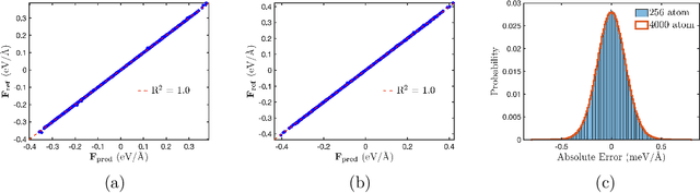
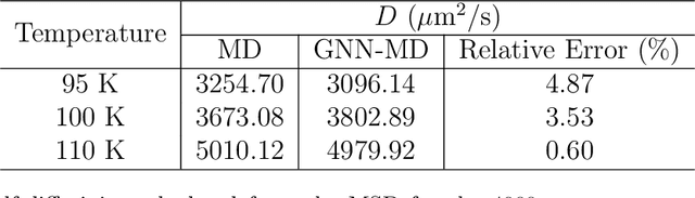
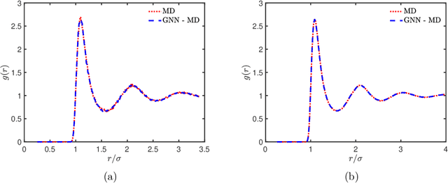
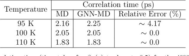
Machine-learned force fields have generated significant interest in recent years as a tool for molecular dynamics (MD) simulations, with the aim of developing accurate and efficient models that can replace classical interatomic potentials. However, before these models can be confidently applied to materials simulations, they must be thoroughly tested and validated. The existing tests on the radial distribution function and mean-squared displacements are insufficient in assessing the transferability of these models. Here we present a more comprehensive set of benchmarking tests for evaluating the transferability of machine-learned force fields. We use a graph neural network (GNN)-based force field coupled with the OpenMM package to carry out MD simulations for Argon as a test case. Our tests include computational X-ray photon correlation spectroscopy (XPCS) signals, which capture the density fluctuation at various length scales in the liquid phase, as well as phonon density-of-state in the solid phase and the liquid-solid phase transition behavior. Our results show that the model can accurately capture the behavior of the solid phase only when the configurations from the solid phase are included in the training dataset. This underscores the importance of appropriately selecting the training data set when developing machine-learned force fields. The tests presented in this work provide a necessary foundation for the development and application of machine-learned force fields for materials simulations.
Understanding Urban Water Consumption using Remotely Sensed Data
May 03, 2022


Urban metabolism is an active field of research that deals with the estimation of emissions and resource consumption from urban regions. The analysis could be carried out through a manual surveyor by the implementation of elegant machine learning algorithms. In this exploratory work, we estimate the water consumption by the buildings in the region captured by satellite imagery. To this end, we break our analysis into three parts: i) Identification of building pixels, given a satellite image, followed by ii) identification of the building type (residential/non-residential) from the building pixels, and finally iii) using the building pixels along with their type to estimate the water consumption using the average per unit area consumption for different building types as obtained from municipal surveys.